Image Processing & Computer Vision Video Series

Hallo teman-teman semuanya! 

Di post ini, saya akan membagikan video series yang akan membahas materi image processing dan computer vision. Video series ini akan membahas detail teorinya, kemudian di sesi berikutnya diikuti dengan praktek implementasi di pemrograman C++ menggunakan libary OpenCV.

Materi diadopsi dari bukunya Gonzales “Digital Image Processing” dari Chapter 1 hingga Chapter 12, yaitu Object Detection, ditambah dengan beberapa topik computer vision, seperti stereo vision. Adapun slide dan code-nya tersedia di link Github di sini. Slide dan code tersebut dapat digunakan secara gratis, baik untuk referensi perkuliahan hingga untuk self-study, dengan tetap mencantumkan sumbernya.

Semoga video series ini membantu teman-teman dalam memahami image processing dan computer vision, dan ikut membantu tumbuhnya iklim science & engineering di Indonesia. Salam 🙂

Apache Spark Tutorial for Big Data Analytics

Hi!

This post will provide you video series talking about how we can do big data analytics using Apache Spark.

Machine Learning from The Scratch using Python

This post provides video series how we can implement machine learning algorithm from the scratch using python. Up to know, the video series consist of clustering methods, and will be continued for regression, classification and pre-processing methods, such as PCA. Check this out!

*this is in playlist mode. So, you can check other videos in the playlist navigation.

Understanding How Mask RCNN Works for Semactic Segmentation

Mask RCNN is extension of Faster RCNN. In 2017, this is the state-of-the-art method for object detection, semantic segmentation and human pose estimation. This awesome research is done by Facebook AI Research.  This post provides video series talking about how Mask RCNN works, in paper review style. May it helps.

1. Introduction to MNC, FCIS ad Mask RCNN for Instance Aware Semantic Segmentation

Understanding Faster R-CNN for Object Detection

Faster R-CNN is important research in object detection. It inspires many other methods how we can do object detection using deep learning, such as YOLO, SSD (Single Shot Detector) and so on. This post provides video series of how Faster RCNN works. The video series is made in paper review style. Hope it helps 🙂

1. Introduction to Faster R-CNN

Understanding Kernel Method/Tricks in Machine Learning

Up to now, we already learn about regression, classification and clustering in our machine learning and pattern recognition post series. During this post, we will learn another powerful method in machine learning, which is kernel method, or also called kernel trick! Why do we use kernel trick? Some reasons are (1) we don’t need to think how to form a design matrix. Just imagine for example if our features are “words”, not number. How can we form design matrix for it? Using kernel method, we can just define our kernel, for example using hamming distance of our “words”, etc. (2) Kernel method provides us a way to project our data into much higher dimensional space, even equals to infinite dimensional space. We can take benefit of it so that our model performs better.

So, how to do kernel trick? We will demonstrate how to do that in our regularized regression. In our regularized regression using LSE we already talk here, we get the loss function to be minimized as follows.

Estimator for Mean and Variance of Sampled Data

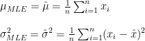
Estimator is a statistic, usually in a function of the data, that is used to infer the value of an unknown parameter in a statistical model. During this post, we will talk about estimator for mean and variance of sampled data. We can determine a good estimator by calculating the bias of it. A good estimator should give bias closed to zero. Let is parameter we want to estimate/observe, our estimator result will be . The bias of our estimator is defined as follows.

We will use bias formula above to check whether our estimator is good or not. And during this post, we will check our estimator we already derived by MLE here, which are mean and variance. Let’s write them first.

where and 

How EM (Expectation Maximization) Method Works for Clustering

Background

To get strong understanding about EM concept, digging from the mathematical derivation is good way for it. But before it, let’s put the condition first. EM method is intended for clustering, and the most familiar method is k-means clustering, which is the special case of EM method that use Gaussian mixture to model the cluster areas and using hard clustering instead of soft clustering.

See picture below.

Picture above shows that we have 4 clusters where each cluster is modeled using Gaussian. To determine the data belongs to which cluster, we can just determine by finding the maximal value among the fourth Gaussian value. The data will be clustered to the cluster whose Gaussian value is maximal in that location. For instance, the area in the pink line boundary has maximal Gaussian value which is from Gaussian value in cluster 1, likewise for other clusters. Doing this type of clustering, the clustering boundary may intersects each others and taking cluster whose the value is maximal, is called soft clustering. Whereas for hard clustering, the boundary doesn’t intersect each others. To be able to cluster like that, we need parameters mean and variance of all those 4 Gaussian distributions, given data set input without class label. And we can achieve this by using EM method.

How Logistic Regression Works for Classification (with Maximum Likelihood Estimation Derivation)

Logistic regression is an extension of regression method for classification. In the beginning of this machine learning series post, we already talked about regression using LSE here. To use regression approach for classification,we will feed the output regression into so-called activation function, usually using sigmoid acivation function. See piture below.

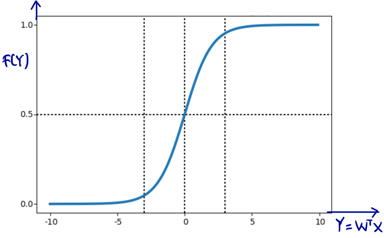
Sigmoid function will have output with s-shape like picture above whose output range is from zero to one. For classification, logistic regression is originally intended for binary classification. Regarding picture above, our output regression is fed sigmoid activation function. We will classify input to when the output is closed to 1 (formally when ) and classify to $class_2$ when the output is closed to 0 (formally when ) To do that, we can achieve by maximizing out likelihood using MLE (Maximum Likelihood Estiamtion).

How k-NN (k-Nearest Neighbors) Works for Classification

We already know that classification problem is predicting given input data into certain class. The simplest and most naive method is nearest neighbor. Given data training with class label, nearest neighbor classifier will assign given input data to the nearest data label. It can be done by using euclidean distance. Here is the illustration.